Exploratory Factor analysis is built on the premise that the variables in your dataset are correlated. If your variables are independent (meaning they don’t share any common variance), factor analysis simply won’t work. You can’t extract a “construct” from variables that have no relationship to one another. Here Bartlett’s Test of Sphericity becomes important to test before moving into factor analysis.
What is Bartlett’s Test of Sphericity ?
Bartlett’s Test of Sphericity is named after the British statistician Maurice Stevenson Bartlett (1910–2002). It’s important in exploratory factor analysis is to ensure variables are sufficiently correlated for meaningful analysis.
Specifically, the test examines your data’s correlation matrix and tests whether it is significantly different from an identity matrix.
You can cite the original paper if you need in your writing as follows (APA):
Bartlett, M. S. (1950). Tests of significance in factor analysis. British Journal of Psychology, 3(1), 77–85.
What is an identity matrix?
An identity matrix is a matrix where all diagonal elements are 1 and all off-diagonal elements are 0. In statistics, if your variables are perfectly correlated with themselves but have a zero correlation with every other variable, your correlation matrix becomes an identity matrix:
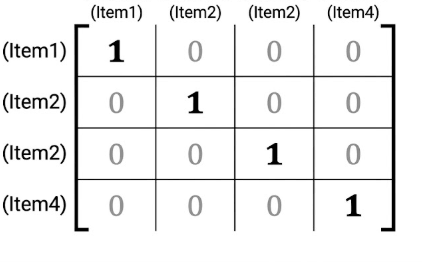
The Rule: If your data’s correlation matrix looks like an identity matrix, your variables are completely unrelated. If they are unrelated, stop immediately. You cannot perform a factor analysis.
Hypothesis Behind the Test
When you run Bartlett’s test, you are performing a formal hypothesis test. Understanding the logic behind these two hypotheses is key to interpreting your software output correctly:
-
Null Hypothesis (): The correlation matrix is an identity matrix.
-
This means that your variables are completely independent of one another. There is no pattern of correlation in your data, and therefore, there is no underlying structure for an Exploratory Factor Analysis to identify. If your results fail to reject this hypothesis, your data is not suitable for EFA.
-
-
Alternative Hypothesis (): The correlation matrix is not an identity matrix.
-
This means that there is at least some degree of correlation between your variables. This is the outcome you are looking for. If you are able to reject null hypothesis, it indicates that the variables share common variance, making them appropriate candidates for factor analysis.
-
How to Run Bartlett’s Test (SPSS, STATA, R)
Please refer the process to run the test in different software as follows:
1. How to Run It in SPSS
SPSS makes this incredibly easy. It pairs Bartlett’s test directly with the KMO measure.
-
Go to Analyze > Dimension Reduction > Factor.
-
Move your variables into the “Variables” box.
-
Click on the Descriptives button.
-
Check the box for KMO and Bartlett’s test of sphericity.
-
Click Continue, then OK. The results will pop up in a neat little table in your output viewer.
2. How to Run It in STATA
In STATA, you typically run this right after a factor analysis or PCA, but you will likely need to install a user-written package first.
* 1. Install the module (you only need to do this once)

ssc install factortest

* 2. Run the test using your specific dataset variables

factortest variable1 variable2 variable3
STATA will show output both KMO and Bartlett’s test results.
3. How to Run It in R
R gives you a lot of flexibility. The most common way to run this is by using the popular psych package.
# 1. Install and load the package (only need to install once)
install.packages("psych")
library(psych)

# 2. LOAD YOUR ACTUAL DATA HERE
# (Example: loading a CSV file named "my_survey_data.csv")
my_data <- read.csv("my_survey_data.csv")

# 3. FILTER FOR NUMERIC COLUMNS
# Bartlett's test only works on numbers. Select only your test variables:
test_variables <- my_data[, c("variable1", "variable2", "variable3")]

# 4. RUN THE TEST
# Method A: Directly using your filtered data
cortest.bartlett(test_variables)

# Method B: Using your data's correlation matrix
cor_matrix <- cor(test_variables, use = "complete.obs") # "complete.obs" handles missing data
cortest.bartlett(cor_matrix, n = nrow(test_variables))
Interpreting the Results
When you run Bartlett’s test, you aren’t looking for a “high” or “low” score in the same way you look at a KMO value. Instead, you are looking for statistical significance.
-
Significant Result (p < .05): You reject the null hypothesis. Your correlation matrix is significantly different from an identity matrix, meaning your variables correlate enough to proceed with EFA.
-
Non-Significant Result (p > .05): You fail to reject the null hypothesis. Your variables are too independent, and factor analysis is inappropriate for this dataset.
Might be helpful: How to Conduct Exploratory Factor Analysis (EFA): 11 Steps Roadmap
Conclusion
Conducting an Exploratory Factor Analysis requires you to prove your data is suitable for that. Bartlett’s Test of Sphericity provides this essential statistical proof. By presenting a significant Bartlett’s test alongside a strong KMO value, you can justify the use of EFA in your dataset.
Reference:
If you need to cite the foundational work in your research paper, use this APA citation:
FAQs
Do I need to report both the KMO and Bartlett’s test in my thesis?
Yes. They measure two different things. KMO measures sampling adequacy (the proportion of variance among your variables that might be common variance), while Bartlett’s tests the correlation matrix itself. Hence, both should be reported .
How to report the results of Bartlett’s test in APA format?
You can report in short like this: “Bartlett’s Test of Sphericity indicated that the correlation matrix was not an identity matrix, chi-square(df = 45) = 321.45, p < .001, confirming that the data is suitable for factor analysis.”