If you are trying to understand what the endogeneity problem in econometrics is, why it matters, and what is its basic example to understand, this post can help. Let’s start our learning.
What Is the Endogeneity Problem?
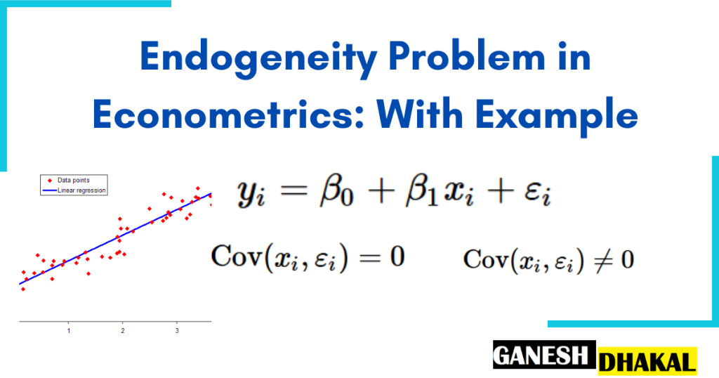
Consider the simple population regression model:
\[y_i = \beta_0 + \beta_1 x_i + \varepsilon_i \]
One of the key assumption for the Ordinary Least Squares (OLS) estimator to be unbiased is the zero conditional mean assumption.
\[ \mathbb{E}[\varepsilon_i \mid x_i] = 0 \]
This means that the expected value of the error term, given the independent variable \(x_i\), should be zero. A slightly relaxed version of this assumption is:
\[ \mathrm{Cov}(x_i, \varepsilon_i) = 0 \]
| Note: If \( \mathbb{E}[\varepsilon_i \mid x_i] = 0 \) holds then \( \mathrm{Cov}(x_i, \varepsilon_i) = 0 \) also holds, but the reverse is not necessarily true. |
In simple terms, the independent variable \(x_i \) should not be correlated with any unobserved factors contained in the error term \(\varepsilon_i \). If this assumption fails, the OLS estimator becomes biased and inconsistent. This issue is what we call the endogeneity problem.
Why Is Endogeneity Problematic?
When \( \mathrm{Cov}(x_i, \varepsilon_i) \ne 0 \) exists, the variation in \(x_i \) includes information about unobserved factors that also influence \(y_i \). As a result, the estimated coefficient \(\beta_1\) will capture not only the effect of \(x_i \) on \(y_i \) but also part of the effect of these omitted or unobserved variables. This leads to biased and misleading conclusions from the model.
Does It Apply to Multiple Regression?
Yes. In a multiple regression model with several explanatory variables, it’s not necessary that all independent variables be endogenous to have a problem. Even if just one independent variable \(x_j \) is correlated with the error term:
\[ \mathrm{Cov}(x_i, \varepsilon_i) \ne 0 \] for some j=1…k (if j=1, it means first independent variable)
the model suffers from endogeneity. So even partial violation of the assumption can compromise the reliability of your estimates.
-
Endogenous variables: those with \( \mathrm{Cov}(x_i, \varepsilon_i) \ne 0 \)
-
Exogenous variables: those with \( \mathrm{Cov}(x_i, \varepsilon_i) = 0 \)
Example of Endogeneity: Education and Wage
A classical example is the relationship between education and wage:
\[wage_i = \beta_0 + \beta_1 education_i + \varepsilon_i \]
One important factor that is not included in the model but may have impact on education and wage is ‘ability’. Since ‘ability’ is not observable and hence now embedded in the error term \(\varepsilon_i \). Individuals with higher ability may both pursue more education and end up with higher wages. So, ability affects both the independent variable (education) and the dependent variable (wage) but is in \(\varepsilon_i \), making:
\[ \mathrm{Cov}(education, \varepsilon) \ne 0 \]
If we omit ability from the model, the estimate of will not reflect the true effect of education alone – it will also include the indirect effect through ability. This makes education an endogenous variable, and the model suffers from endogeneity.
Causes of Endogeneity
Common causes of endogeneity include:
- Omitted variable bias (as in the example above)
- Simultaneity (when and influence each other
- Measurement error in the independent variable
Conclusion
Endogeneity is a common and serious issue in regression analysis. When an explanatory variable is correlated with the error term, the results of your model can no longer be trusted. Understanding the causes and using appropriate methods to deal with it is key to building credible econometric models.